

This exercise demonstrates how to use HydroDesktop to find and analyze water data for Jacob’s Well Spring in Texas. With some simple analysis, you will compare characteristics of this groundwater-dominated system with those of a nearby river. During the exercise, you will learn about some of the most commonly-used tools in HydroDesktop.
Credit: This exercise was developed by Tim Whiteaker (University of Texas at Austin) and David Tarboton (Utah State University).
On this Page:
About Jacob's Well
Exercise Procedure
Advanced: Analysis with R
The underwater cave known as Jacob’s Well emerges in Hays County, Texas, at Jacob’s Well Spring where it serves as one of the primary sources of water for Cypress Creek, which later flows into the Blanco River. The clear, crisp water cools down many Texans as it moves through the Blue Hole swimming area near Wimberley, Texas. This karst spring has been impacted in recent years by development in Hays County and increasing demands on the Middle Trinity Aquifer (Davidson, 2008).
 |
Jacob's Well Spring (San Marcos Local News, 2009)
|
In 2005, a monitoring station was installed at Jacob’s Well Spring 18 meters below the ground surface, reporting flow and temperature conditions at 15-minute intervals. The data for this station are accessible via the US Geological Survey’s National Water Information System (USGS NWIS).
 |
Jacob's Well Spring Monitoring Station (United States Geological Survey, 2007)
|
For more information about the spring, please read the 2008 Masters thesis of Sarah Cain Davidson from The University of Texas at Austin.
Goals and Objectives
The goal of this exercise is to introduce you to the tools and functions available in HydroDesktop that allow you to search for and synthesize hydrologic time series data in an area of interest. This exercise will teach you how to find and obtain data for Jacob’s Well Spring in Texas and compare data characteristics using the analysis capabilities of HydroDesktop.
Objectives for this exercise include:
• Find streamflow and temperature data for Jacob’s Well Spring in Texas.
• Identify useful time series and download them.
• Visualize time series data in graphs.
• Export time series data for use in other programs.
Suppose you live in Hays County in Texas, and for years you have enjoyed taking a dip in the Blue Hole swimming area along Cypress Creek during hot Texas summers. As population growth and increased groundwater pumping threaten Jacob’s Well Spring, the primary source of water for Cypress Creek, you decide to learn more about this valuable resource. In this exercise, you’ll use HydroDesktop to find temperature data and see how it compares to a nearby river.
The county boundary for Hays County is included in the U.S. Counties layer that is already in the map. You’ll use this boundary to restrict the area being searched.
To search for streamflow in Hays County:
1. Set the context with an online basemap.
- (A) On the Map tab, in the Online Basemap panel, choose a basemap such as ESRI World Topo.
- (B) In the Online Basemap panel, set the Opacity of the basemap to 50.
- (C) In the Legend, uncheck the U.S. States layer to hide that layer.
2. In the ribbon, click the Search tab.
3. Select Hays County as the area of interest.
- (A) In the Area panel on the ribbon, click Select by Attribute.
- (B) Select U.S. Counties as the active layer. The default field of NAME will suffice.
- (C) Select Hays, TX, from the list of county names. You can click in the list and start typing “Hays” to quickly find the item you’re looking for.
- (D) Click OK.
 |
Choosing a
Search Area
|
Next you will tell HydroDesktop what hydrologic variables you want. To help you in this regard, HydroDesktop employs a list of official CUAHSI-HIS keywords for hydrologic variables. Data providers use this list when registering with CUAHSI-HIS. This is a lot easier than typing whatever term the data provider may be using internally (e.g.,
00060 for USGS streamflow).
4. In the box within the Keyword panel on the ribbon, type Streamflow. The box bottom box autocompletes to a valid search term from the list of parameter keywords that CUAHSI maintains while the top box allows freeform entries.
Next you will tell HydroDesktop the date range of time series that you want. For this exercise, search for data available in the 2010 water year, i.e., 10/1/2009 to 9/30/2010.
5. In the Time Range panel, change the start date and end date to 10/1/2009 and 9/30/2010, respectively.
 |
The Search tab displays your search criteria as you enter them
|
At this point you could click in the Data Sources panel to restrict the search to specific data sources, but for this portion of the exercise you will search all data sources, which is the default setting. With search parameters set, you will now tell HydroDesktop to run the search for data.
6. In the Search panel, click Run Search.
7. Once the search has completed, close the progress dialog.
When you run a search, HydroDesktop asks the CUAHSI-HIS national catalog for descriptions of time series that match your search criteria. At this point, your software is using a remote online resource and bringing back information to display in your map. After HydroDesktop has finished searching for time series, it displays the locations of time series that fit your search criteria in a map layer called Data Sites. Different symbols for the sites indicate different data sources. You can see a label for the Jacob’s Well Spring site in the map.
 |
| Locations of Streamflow in Hays County |
While the search may have seemed fast, remember that your map is only showing where time series of interest are located, and that you haven’t actually downloaded any time series values yet. Now you can begin to refine these search results to locate time series that you actually want to download and save to your database.
Downloading Data
For this exercise, you will work with streamflow at the following two sites:
- Jacobs Well Spg nr Wimberley, TX
- Blanco Rv nr Kyle, TX (a site near Jacob’s Well Spring for comparison)
You will select the features that represent these time series so that HydroDesktop knows which time series you want to download. While several data sources were returned from the search, in this exercise you will only download streamflow from the USGS National Water Information System Daily Statistics archive (NWIS Daily Values).
To select time series for download:
1. In the Legend on the left, uncheck all layers except for the NWIS Daily Values to hide those layers. The only layer you will work with is the NWIS Daily Values layer.
2. Right-click the NWIS Daily Values layer name and click Attribute Table Editor.
The Attribute Table Editor opens showing you descriptions of time series in this layer. You can scroll through the table and resize columns to see the information.
3. In the Attribute Table Editor, use the values in the SiteName and VarCode columns to identify time series of average streamflow values for the two sites listed above. While holding down the CTRL key, left-click on these rows to select them.
 |
Selecting Time Series for
Download
|
4. Close the Attribute Table Editor.
With these rows selected, you are ready to download the data.
5. In the ribbon, in the Search panel, click Download. The Download Manager opens to show progress of the download.
 |
The Download Manager
|
6. Hide the Download Manager when the download is complete.
Tip: If a download fails, you can right-click the failed row in the Download Manager to attempt the download again.
Downloading Additional Data
You might be excited about viewing your downloaded data, but before you do, let’s retrieve some water temperature data for Jacob’s Well Spring. Since you retrieved data from NWIS Daily Values in the previous search, you will learn how to restrict a search so that NWIS Daily Values is the only data source that is queried.
To search for and download water temperature data:
1. In the ribbon, in the Keyword panel, enter Water temperature in the bottom (autocomplete) box.
2. Restrict the search to NWIS Daily Values.
(A) In the Data Sources panel, click All Data Sources.
(B) In the Data Sources dialog, click Select None.
(C) In the list of data sources, find and place a check next to NWIS Daily Values.
(D) Click OK to close the Data Sources dialog.
Tip: You can click the name of a data source in the Data Sources dialog to open a Web page with more information about that source.
 |
| Choosing Data Sources |
Notice how the icon for All Data Sources has changed to reflect the chosen data source.
3. In the Search panel, click Run Search.
4. Once the search has completed, close the progress dialog.
An NWIS Daily Values (2) layer is added to the map legend to show results from this second search.
5. In the Legend on the left, right-click the NWIS Daily Values (2) layer name and click Attribute Table
Editor.
6. In the Attribute Table Editor, use the values in the SiteName and VarCode columns to identify time series of average temperature values for these two sites:
- (A) Jacobs Well Spg nr Wimberley, TX
- (B) Blanco Rv at Halifax Rch nr Kyle, TX
7. While holding down the CTRL key, left-click on these rows to select them.
8. Close the Attribute Table Editor.
9. In the ribbon, in the Search panel, click Download.
10. Hide the Download Manager when the download is complete.
Now that you’ve downloaded the data, you can view the data in both tabular and graph form.
Visualizing Time Series Data
HydroDesktop takes a series-centric view of temporal data, meaning that it provides access to the data at the time series level. An example of a time series is all of the temperature values measured at a certain point on the Blanco River. Let’s take a look at the time series that you just downloaded.
To visualize time series data in HydroDesktop:
1. Click the Graph tab in the ribbon to activate it.
On the left you will see a list of all the time series in your database. You could use filters to restrict the time series
that are shown, but you only retrieved a handful in this exercise so it’s fine to leave the default view.
2. In the list of time series on the left, place a check next to temperature at the Blanco River at Halifax
Ranch.
From the graph you can see how the temperature in the water changes with the seasons throughout the year.
Now let’s compare this time series with the one for Jacob’s Well Spring.
3. Place a check next to temperature at Jacob’s Well Spring.
HydroDesktop allows you to visualize multiple time series on the same graph. The plot axes automatically adjust to fit your data. In this example, there is a dramatic difference between the two temperature time series. The one for Jacob’s Well Spring shows much less variation throughout the year than the one for the Blanco River at Halifax Ranch.
 |
Comparing Temperature Time Series
|
4. In the ribbon, click Probability to show a probability plot of the data, further illustrating the difference between the two time series.
5. Click TimeSeries to restore the time series view.
The dramatic difference in the shapes of the two time series plots is caused by the source of water for these two rivers. The Blanco River at Halifax Ranch is largely a surface water system while Jacob’s Well Spring is fueled by groundwater. While the groundwater system does maintain a much more steady temperature than the surface water system, notice how jumps still exist, such as the sudden decrease in temperature in mid-January, 2010. Let’s plot flow on this graph to see why this might be happening.
6. Place a check next to Discharge at Jacob’s Well Spring.
Notice the sharp increase in streamflow around the same time that the water temperature dropped. It seems like the system is experiencing a large influx of surface water, which is colder than the groundwater in the winter. Similarly, you can see an increase in streamflow in late summer, 2010, which results in an increase in water temperature.
 |
| Examining Changes in Flow and Temperature |
7. Uncheck the two temperature time series, and place a check next to Discharge at the Blanco River near Kyle.
The flow of the Blanco River dwarfs that of Jacob’s Well Spring, but you can still see increases in flow in the Blanco River at about the same time as those observed in the spring. Also notice the peak flow in September, 2010. This flow is the result of tropical storm Hermine as it swept through Texas.
Delineating Watersheds
At this point, it might be nice to see precipitation data in this watershed for this water year. You can delineate watersheds for any river in the conterminous U.S. using a Web service provided by the EPA. All you have to do is click on the desired watershed outlet location in the map, and then HydroDesktop sends that point location to the EPA service. The service figures out which National Hydrography Dataset (NHD) reach the clicked point is closest to, and then finds all catchments that the reach drains. The catchments are merged into a single watershed and returned to HydroDesktop.
Note that the watershed returned is for the outlet of the entire reach, so if the point you clicked isn’t at the reach outlet, then the resulting watershed will include some additional area downstream of your clicked point. Thus, this tool is useful for helping to identify an area of interest but should not be used to determine watershed parameters such as area. Future versions of the tool will support more precise delineation.
In this portion of the exercise you will delineate a watershed for the area draining to Jacob’s Well Spring. The watershed delineation tool is part of a HydroDesktop extension called EPA Delineation.
To delineate a watershed for the area draining approximately to the Jacob’s Well Spring location:
1. On the Map tab, in the Zoom panel, activate the (zoom) In tool. Draw a box around the site at
Jacob’s Well Spring to zoom in to it a bit. This helps ensure that you click exactly at the spring outlet.
2. In the Legend, uncheck U.S. Counties to hide that layer.
3. In the EPA Tool panel, click Delineate to activate the delineation tool.
4. The tool prompts you for where to save the resulting datasets. Accept the defaults by clicking OK.
5. Click on the site location for Jacob’s Well Spring.
After a moment, the watershed is shown in the map. The NHD reaches flowing to the point that you clicked and the point itself are also shown.
 |
| Delineated Watershed |
If you didn’t get the correct watershed delineated then you can activate the tool and try again. It’s OK to overwrite
previous results.
Note: Recall that the watershed is actually delineated for the outlet of the nearest NHD reach, which happens to be very close to Jacob’s Well Spring in this example. Also be aware that the surface watershed you just delineated defines some but not all of the area contributing water to the aquifer for Jacob’s Well Spring. However, the area will suffice for this exercise which merely demonstrates how to delineate watersheds and use those watersheds to find data.
With the watershed delineated, now you’re ready to search for data in this watershed.
Finding Data in a Watershed
Now you’ll search for daily precipitation data from the National Weather Service (NWS) in the watershed for Jacob’s Well Spring.
1. In the ribbon, click the Search tab.
2. Choose the delineated watershed as the area of interest.
- (A) Click Select by Attribute, which is located in the area section of the Search tab.
- (B) Select Watershed as the active layer. The default field of Id will suffice.
- (C) Select the only value present, which is probably a value of 1.
- (D) Click OK.
3. In the Keyword panel, enter Precipitation.
4. Restrict the search to the NWS West Gulf River Forecast Center’s (WGRFC) multi-sensor precipitation estimates.
- (A) In the Data Sources panel, click the currently selected data source, NWIS Daily Values.
- (B) In the Data Sources dialog, click Select None.
- (C) In the list of data sources, find and place a check next NWS-WGRFC Daily Multi-sensor
- Precipitation Estimates.
- (D) Click OK to close the Data Sources dialog.
5. In the Search panel, click Run Search.
6. Once the search has completed, close the progress dialog.
When the search finishes, you’ll see some regularly-spaced dots over the watershed. These dots represent the centroids of NEXRAD HRAP cells. In other words, this Web service provides discrete point locations where you can basically sample this gridded rainfall dataset. Each of these points is like a virtual rain gauge. For this exercise, you’ll just pick one near Jacob’s Well Spring.
In addition to choosing time series from the Attribute Table Editor as you have already done in this exercise, you can also hover your mouse over a site and download time series from the pop-up bubble that appears.
7. Hover your mouse over one of the precipitation sites.
8. In the pop-up bubble that appears, click Download.
 |
| Popup windows summarize time series available at a given location |
9. Hide the Download Manager when the download is complete. The precipitation data are added to your database.
Now let’s view the results.
1. Click the Graph tab.
2. Plot a graph with one of the precipitation time series you just downloaded and Streamflow from
Jacob’s Well Spring. Notice how quickly Jacob’s Well Spring responds to rainfall events.
 |
| Precipitation and Streamflow at Jacob's Well Spring |
While HydroDesktop does contain additional analysis capabilities, it can also export data to a text file for use in other programs.
Exporting Data
HydroDesktop can export data to a variety of output file types for further study and analysis. For example, you can export individual time series by right-clicking them in Table or Graph view. For this exercise, you will export all time series that you have downloaded.
To export time series data:
1. Click the Table tab in the ribbon to activate it.
2. In the Data Export group, click Export.
This tool exports data to a delimited text file. In the Export To Text File dialog, notice that the time series are organized into “data sites” layers. Each “data sites” layer corresponds to a given data source and search parameter. You can choose to only export data for a given data source if desired. You can also control the fields that are included in the export and choose a delimiter. For this exercise, you will accept all defaults to produce a comma delimited text file.
 |
Export To Text File Dialog
|
3. In the Export To Text File dialog, specify the output file location and name.
4. Click Export Data.
5. Close the Export To Text File dialog when it is finished.
6. Find the file on your computer and open it to verify that the data were exported.
Congratulations! With your data in hand, you have completed the exercise and learned how to use HydroDesktop to discover and access water data. Feel free to experiment with other functionality such as creating and printing a map, and be sure to give feedback using the Help tab. This concludes the main portion of the exercise. For an example of more advanced analysis, continue with the section below to learn how to use the R statistical environment with HydroDesktop.
The work above has illustrated how to download temperature, precipitation and discharge data and suggested that variations in temperature in Jacob's Well Spring may be related to the mixing of surface and subsurface water sources. In this section, you will use the HydroR plug-in in HydroDesktop to explore this phenomenon. The HydroR plug-in provides an interface between HydroDesktop and the free R statistical software environment.
Enabling HydroR
Once R is installed, you will need to enable HydroR in HydroDesktop.
To enable HydroR:
1. Click the HydroR tab in the ribbon.
2. In the HydroR Tools panel, click Start R.
3. If prompted for the path to R.exe, enter the path where it was installed on your computer. Note that R may include more than one R.exe file. The one you typically need is in the bin\i386\ folder, as in C:\Program Files\R\R-2.13.0\bin\i386\R.exe. Click OK once the path is entered. HydroDesktop will remember this path the next time you use the HydroR extension.
4. HydroDesktop needs some additional R libraries. If you are using the HydroR extension for the first time, you may be prompted for a CRAN mirror to download these libraries. Select the mirror closest to your location and click OK. The appropriate libraries are downloaded automatically.
R should now start and give you a blank R script in the top panel and R Console in the bottom panel. Standard R commands can be entered in the R Console. HydroR makes it easy to provide R access to the data you have downloaded with HydroDesktop using the HydroR tab.
 |
HydroR Layout
|
Plotting a Graph with R
To get familiar with how HydroR works, you’ll plot a hydrograph for Jacob’s Well Spring.
To plot a graph in HydroR:
1. In the HydroR tab, in the list of time series on the left, select a time series that you would like to import as a data frame into R. For this exercise, select discharge at Jacob’s Well Spring. Make sure no other time series are selected.
2. In the ribbon, click Generate R code. The R code to get the selected data series is entered into the script.
3. Click Send All. This sends the script text to the console and executes it. The result is an object named
data0, which contains a list of R data frames.
4. In the R Console, enter labels(data0) to see a list of data frames that make up data0.
These data frames are basically tables from your HydroDesktop database. The key table we’re interested in for this exercise is the DataValues table.
5. To see the first few rows of DataValues, in the R Console, enter head(data0$DataValues) (R is case sensitive, so type the command exactly as it appears in this text). You may have to scroll up in the R Console to see the full result.
You’ll use the LocalDateTime and DataValue columns to provide data for the graph.
6. To make it easier to access this streamflow time series, in the R Console, enter Q.jacobs=data0$DataValues. This assigns the DataValues data frame to a variable named Q.jacobs.
7. In the R Console, enter plot(Q.jacobs$LocalDateTime,Q.jacobs$DataValue,type="l") (the type is a lower case L, not a one). A time series plot of the data should appear in an R graphics window, demonstrating that the full capability of R is available to work with the data that has been imported.
 |
Jacob’s Well Spring Hydrograph Plotted Using R
|
Let’s add a title to this graph.
8. In the R Console, enter data0$Variable to see all attributes for the Variable table.
9. In the R Console, enter title(data0$Variable$VariableName) to add the variable name as the title for the plot.
10. After verifying that the title was added, close the R graphics window showing the graph.
Analyzing Flow in Jacob's Well Spring
Let's use mixing theory to estimate the fractions of Jacob's Well Spring flow that are from the surface and subsurface based on temperature. Assume the surface source has temperature equal to the temperature in Blanco River. Assume groundwater source is at a fixed temperature. The following equations then apply.
Energy Balance: QT=Q1T1+Q2T2
Mass Balance: Q=Q1+Q2
where Q is discharge in Jacob's Well Spring, T is Temperature in Jacob’s Well Spring, T1 is the temperature of the surface source (assumed equal to Blanco River temperature), and T2 is the temperature of the subsurface source (assumed constant and taken as the average of last 60 days). Q1 and Q2 are the unknown discharge contributions from surface and subsurface sources respectively (Figure 22).
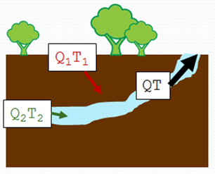 |
Surface
and subsurface contributions to Jacob's Well Spring outflow and temperature
|
Two linear equations, two unknowns can be easily solved (see your high school algebra book). The solution is
Q1/Q = (T-T2)/(T1-T2)
The R scripts in Appendix A use data from HydroDesktop to solve this equation. You’ll assign the relevant time series to simple variable names and then use the R scripts to plot a graph representing the amount of flow in Jacob’s Well Spring inferred as coming from the surface.
To use the R scripts to compute fractional flow:
1. In the same manner that you created the Q.jacobs variable above and assigned it to be the discharge at Jacob’s Well Spring, create and assign the following R variables (remember, the variable names are case sensitive). In other words, for each variable, clear the R script panel, select a series, generate
the R code, send it to R, and assign the variable in the R Console.
- (A) Q.blanco – Discharge at the Blanco River near Kyle
- (B) t.blanco – Water temperature at the Blanco River at Halifax Ranch
- (C) t.jacobs – Water temperature at Jacob’s Well Spring**
**Important: You may encounter a bug when generating R code for water temperature at Jacob’s Well Spring. In the R script panel, if the endDate is not “2010-09-30” then edit the script to use “2010-09-30” before sending the script to the R Console.
2. Enter Script 1 found in Appendix A into the R Console to execute the script. This script prepares inputs for the analysis and plots graphs of the input temperature and flow.
3. Once you have reviewed the graphs of temperature and streamflow generated by Script 1, close the two R Graphics Windows containing the graphs.
4. Enter Script 2 found in Appendix A into the R Console to execute the script. This script smoothes the temperature time series and then performs the analysis to determine the fraction of flow in Jacob’s Well Spring from surface water.
The resulting graphs show smoothed temperature time series and the portion of flow in Jacob’s Well Spring inferred to be from the surface (the red line in the graph). Note that the analysis requires differences between the assumed groundwater temperature and surface water temperature, so the graph will be missing segments when those temperatures are nearly the same.
|
Fractional Flow in Jacob's Well Spring
|
Congratulations! You have completed the exercise and seen how advanced analysis environments such as R can be integrated into HydroDesktop using the power of plug-ins. This concludes the advanced portion of the exercise.
Script 1: Preparing Inputs for Flow Analysis
# Script 1: Preparing Inputs for Flow Analysis
# This code plots input time series of flow and temperature.
# The code assumes the following variables have already been set to
# the DataValues data frame for these time series:
# Q.jacobs - Discharge at Jacob's Well Spring
# Q.blanco – Discharge at the Blanco River near Kyle
# t.jacobs – Water temperature at Jacob’s Well Spring
# t.blanco – Water temperature at the Blanco River at Halifax Ranch
# The code handles intermittent missing values
# Start one day earlier because queries seem to be based on UTC
DT = seq(from=as.Date("2009-09-30"),to=as.Date("2010-09-30"),by=1)
ind=match(as.Date(t.blanco$LocalDateTime,"%Y-%m-%d %H:%M:%S"), DT)
T1=rep(NA,length(DT)) T1[ind]= t.blanco$DataValue
ind=match(as.Date(t.jacobs$LocalDateTime,"%Y-%m-%d %H:%M:%S"), DT) T=rep(NA,length(DT))
T[ind]=t.jacobs$DataValue
T2 = T[1] # The first value
ind=match(as.Date(Q.jacobs$LocalDateTime,"%Y-%m-%d %H:%M:%S"), DT) Q=rep(NA,length(DT))
Q[ind] = Q.jacobs$DataValue
plot(DT,T1,type="l",ylab="T")
lines(DT,T,col=2)
legend("bottomright",c("T Blanco","T Jacobs"),col=c(1,2),lty=1)
windows()
plot(DT,Q,type="l")
Script 2: Computing Surface Water Flow Fraction
# Script 2: Computing Surface Water Flow Fraction
# This script solves the equation Q1/Q = (T-T2)/(T1-T2)
# and plots a graph showing the portion of flow inferred
# to be directly from surface water sources in Jacob’s
# Well Spring.
# Before running this script, you must run SCRIPT 1:
# PREPARING INPUTS FOR FLOW ANALYSIS
# Smoothing Blanco River temperature data using lowess
ind=!is.na(T1) # array indices of unmissing values
T1l<-lowess(DT[ind],T1[ind],f=0.1)
plot(DT,T1,type="l",ylab="Degrees C")
lines(T1l,col=2)
lines(DT,T,col=3)
legend("bottomright",c("Blanco T","Smoothed Blanco T","Jacobs T"),col=c(1:3),lty=1)
title("Temperatures")
# Match the dates of the output for use in calculations
ind=match(T1l$x,DT)
T1s=rep(NA,length(DT))
T1s[ind]=T1l$y
# For results to be reasonable T1 and T2 have to be different.
# Only evaluate answers when T1 and T2 differ by at least 3 degrees
# Also only accept positive answers
# Calculate T2 as average over last 60 days
T2p=c(rep(T[1],59),T)
T2=rep(NA,length(DT))
for(i in 1:length(DT)) T2[i]=mean(T2p[i:(i+59)],na.rm="True")
Q1f=(T-T2)/(T1-T2) # apply the mixing solution equation
# eliminate answers when temperature difference is less than 3
indna=abs(T1-T2)<3
Q1f[indna]=NA
indna=Q1f< -0.05 # eliminate large negative values
Q1f[indna]=NA
# Plot the results
windows()
plot(DT,Q,type="l",ylab="cfs",lwd=2)
lines(DT,Q*Q1f,col=2,lwd=2)
legend("topright",c("Flow","Inferred From Surface"),lty=1,col=c(1,2))
title("Jacob's Well Discharge")
References
Davidson, S. C. (2008). Hydrogeological characterization of baseflow to Jacob’s Well spring, Hays County, Texas (Master’s thesis). Retrieved November 2, 2010, from Hays Trinity Groundwater Conservation District Web site: http://haysgroundwater.com/files/Documents/Davidson-08_thesis_Cypress_Crk_Jacobs_Well.pdf
San Marcos Local News. (2009, March 10). Jacobs Well area to hold incorporation vote. Retrieved November 2, 2010, from San Marcos Local News Web site: http://www.newstreamz.com/2009/03/10/area-around-jacobs-well-to-hold-incorporation-election/.
United States Geological Survey. (2007, March 26). National Surface Water Conference and Hydroacoustics Workshop. Retrieved November 1, 2010, from United States Geological Survey Web site: http://water.usgs.gov/osw/images/2007_photos/Hydroacoustics.html.